lightray_index.. _annotated-example:

Annotated Example¶

To understand how salsa works and what it can do, here is an annotated example to walk through a use case of salsa.

Extracting Absorbers¶

One of the main goals of salsa is to make it easy to construct a catalog of absorbers that can then be further analyzed. The process of constructing absorbers takes two steps.

Step 1: Generate Light Rays¶

trident is used to generate light rays that pass through your simulation. These are 1-Dimensional objects that connect a series of cells and save field information contained in those cells, ie density, temperature, line of sight velocity. From these we can then extract absorbers along these light rays. (for further information see trident’s documentation)

To aid in generating these light rays, salsa contains the generate_lrays function which can generate any number of lightrays which uniformly, randomly sample impact parameters. This gives us a sample that is consistent with what the sample of observational studies. This prevents any sampling bias when doing comparisons.

To get started we need to get a dataset. The one used in this example can be found here

To use this function first create a directory to save rays::

$ mkdir my_rays

Now we can load in a data set and define some of the parameters that we will look for.

import yt
import salsa
import numpy as np
import pandas as pd

# load in the simulation dataset
ds_file = "HiresIsolatedGalaxy/DD0044/DD0044"
ds = yt.load(ds_file)

# define the center of the galaxy
center= [0.53, 0.53, 0.53]

# the directory where lightrays will be saved
ray_dir = 'my_rays'
n_rays=4

# Choose what absorption lines to add to the dataset as well as additional
# field data to save
ion_list=['H I', 'C IV', 'O VI']
other_fields = ['density', 'temperature', 'metallicity']

# the maximum distance a lightray will be created (minimum default to 0)
max_impact = 15 #kpc

With the parameters set up we can now generate the lightrays. We will set the seed used to create the random light rays so we can reproduce these results.

# set a seed so the function produces the same random rays
np.random.seed(18)

# Run the function and rays will be saved to my_rays directory
salsa.generate_lrays(ds, center, n_rays, max_impact,
                     ion_list=ion_list, fields=other_fields, out_dir=ray_dir)

Step 2: Extract Absorbers¶

For more details on absorber extraction see Absorber Extraction. But the quick synopsis is there is the SPICE method and the Spectacle method. SPICE looks at cell level data while Spectacle fits lines to a synthetic spectra that is generated by trident. The AbsorberExtractor class can use both methods.

Now let’s extract some absorbers from the Light rays we made

ray_file = f"{ray_dir}/ray0.h5"

# construct absorber extractor
abs_ext = salsa.AbsorberExtractor(ds, ray_file, ion_name='H I')

# use SPICE method to extract absorbers into a pandas DataFrame
units_dict=dict(density='g/cm**3', metallicity='Zsun')
df_spice = abs_ext.get_spice_absorbers(other_fields, units_dict=units_dict)
df_spice.head()

name	wave	redshift	col_dens	delta_v	vel_dispersion	interval_start	interval_end	density	temperature	metallicity
H I	1215.670	0.000	12.787	14.187	0.384	201	204	0.000	96469.462	1.086
H I	1215.670	0.000	15.367	-0.264	4.846	204	216	0.000	48429.090	1.103

Can also extract using Spectacle:

# use spectacle now
df_spect = abs_ext.get_spectacle_absorbers()
df_spect.head()

name	wave	col_dens	v_dop	delta_v	delta_lambda	ew	dv90	fwhm	redshift
HI1216	1215.670	15.154	31.705	-5.915	0.000	7.759	40.000	0.217	0.000

Notice that both of these methods contain different information. SPICE includes more details of the simulation data like the density and temperature of the absorber, something that is not easily detected from the spectra. Spectacle contains more information of the line like the equivalent width and the doppler b parameter.

To extract absorbers from multiple LightRays you can use the get_absorbers function. This will loop through a list of rays and extract absorbers from each one. see::

ray_list = [f"{ray_dir}/ray0.h5",
            f"{ray_dir}/ray1.h5",
            f"{ray_dir}/ray2.h5",
            f"{ray_dir}/ray3.h5"]

# initialize a new AbsorberExtractor for looking at C IV
abs_ext_civ = salsa.AbsorberExtractor(ds, ray_file, ion_name='C IV')
df_civ = salsa.get_absorbers(abs_ext_civ, ray_list, method='spice',
                       fields=other_fields, units_dict=units_dict)

df_civ.head()

name	wave	col_dens	delta_v	vel_dispersion	interval_start	interval_end	temperature	metallicity	lightray_index
C IV	1548.187	14.057	-2.221	13.672	201	224	53985.906	1.103	0
C IV	1548.187	13.596	116.462	6.576	110	125	29972.846	1.107	2
C IV	1548.187	13.625	115.329	3.075	139	155	34632.022	1.101	2

Notice that the Spectacle method could also be used. Also, although the AbsorberExtractor takes a ray file at construction, new rays can be loaded into it.

To retain information on where each absorber came from, an lightray_index is given. The number represents the ray it was extracted from. So all absorbers extracted from ray2.h5 would have an index of 2. This can be useful for comparing/analyzing absorbers on the same sightline.

Catalog Generation¶

To generate a full catalog of absorbers we can use the generate_catalog function to both generate a sample of trident.LightRay objects and then AbsorberExtractor to extract absorbers of a list of ions.

Here is what you need to setup and run::

df_catalog = salsa.generate_catalog(ds, n_rays, ray_dir, ion_list,
                                    fields=other_fields, center=center,
                                    impact_param_lims=(0, max_impact),
                                    method='spice', units_dict=units_dict)

df_catalog.head()

name	wave	col_dens	delta_v	vel_dispersion	interval_start	interval_end	temperature	metallicity	absorber_index
H I	1215.670	18.678	108.065	1.509	107	156	16302.538	1.096	2
H I	1215.670	12.787	14.187	0.384	201	204	96469.462	1.086	0
H I	1215.670	15.367	-0.264	4.846	204	216	48429.090	1.103	0
C IV	1548.187	13.596	116.462	6.576	110	125	29972.846	1.107	2
C IV	1548.187	13.625	115.329	3.075	139	155	34632.022	1.101	2
C IV	1548.187	14.057	-2.221	13.672	201	224	53985.906	1.103	0

This function looks first to see if rays have been created in the given directory. If there are the right number of rays and they all contain the right ions and other fields that were specified (in this case that would be ‘density’, ‘temperature’, ‘radius’), then those rays will be used. Otherwise, new rays are created using generate_lrays.

Next, get_absorbers is used to find the absorbers from each ion in ion_list and finally a catalog is returned as a pandas.DataFrame. Note that the lighray index is unique only up to the ion/wavelength

Visualizing Absorbers¶

To visualize what is actually be extracted from the LightRay objects and synthetic spectra, you can use the AbsorberPlotter class. This is built off of the AbsorberExtractor with added functionality to make plots.

To get a full picture of what is happening at each level we can create a multi panel plot containing:

a slice of the simulation with the ray annotated

The number density profile along the ray’s path

The line of sight velocity profile along the ray’s path

The synthetic spectra created from the ray

This figure gives you a good overview of what is happening and can give valuable context to the absorption extraction methods. Additionally, each plot can be made individually if you care less about the spectra, or don’t want to plot a slice (which can be time consuming, depending on the detail in the simulation).

To create the multi-panel plot::

import salsa
import yt
import matplotlib.pyplot as plt

# set the dataset path and load the light ray
ds_file="HiresIsolatedGalaxy/DD0044/DD0044"
ray = yt.load("my_rays/ray0.h5")

# set the y limits for one of the plots
num_dense_min=1e-11
num_dense_max=1e-5
plotter = salsa.AbsorberPlotter(ds_file, ray, "H I",
                                center_gal=[0.53, 0.53, 0.53],
                                use_spectacle=True,
                                plot_spectacle=True,
                                plot_spice=True,
                                num_dense_max=num_dense_max,
                                num_dense_min=num_dense_min)

fig, axes = plotter.create_multi_plot(outfname='example_multiplot.png')

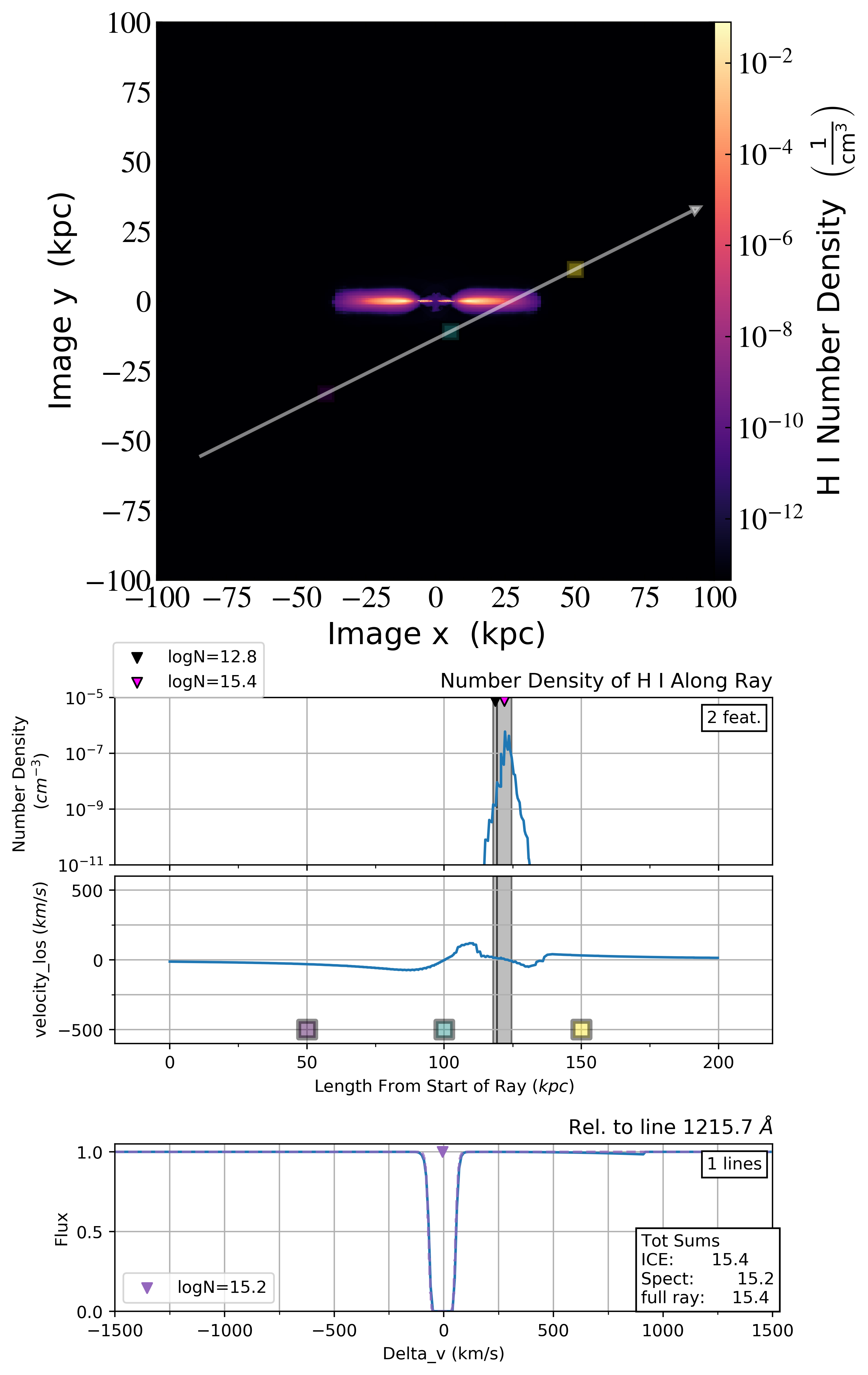
The grey regions on the middle two plots indicate the absorbers that the SPICE method finds. The three highest column densities are marked and displayed in a legend. In the last plot, the solid lines indicate the “raw” spectra while the dotted lines show the absorption lines that Spectacle fit (only the three largest lines are plotted with their column densities recorded in a legend).

The total column density along the lightray, the total found via the SPICE method and the total found by Spectacle is recorded in a legend in the spectra plot.

You can see there is a discrepancy between the SPICE and Spectacle method. Due to the changing velocity profile, the SPICE method extracts two absorbers. Spectacle only fits one absorber because the larger absorber drowns out the smaller one.