Absorber Extraction Methods

The main purpose of SALSA is to extract absorbers from Trident LightRays. Doing this allows us to create synthetic absorption line catalogs/surveys in an analogous fashion as real observational surveys. As of version ???, the only supported extraction method is the SPICE method, which looks directly at cell level data of the simulation. The SPICE algorithm is described in detail below.

SPICE Method

The SPICE (Simple Procedure for Iterative Cloud Extraction) method looks at a Trident LightRay and attempts to extract “absorbers” by identifying contiguous groups of cells along the ray that will contribute to observable features in the absorption spectra.

The algorithm that does this is an iterative process and for a more detailed and likely easier to comprehend explanation see Detailed Example. But here is a rundown of how the algorithm functions to extract absorbers from a light ray

Quick rundown of SPICE method:

1.) Find cutoff in number density such that 80% of the column density is contained in cells with number density above this threshold.

2.) Define intervals that encompass the cells which meet this cutoff.

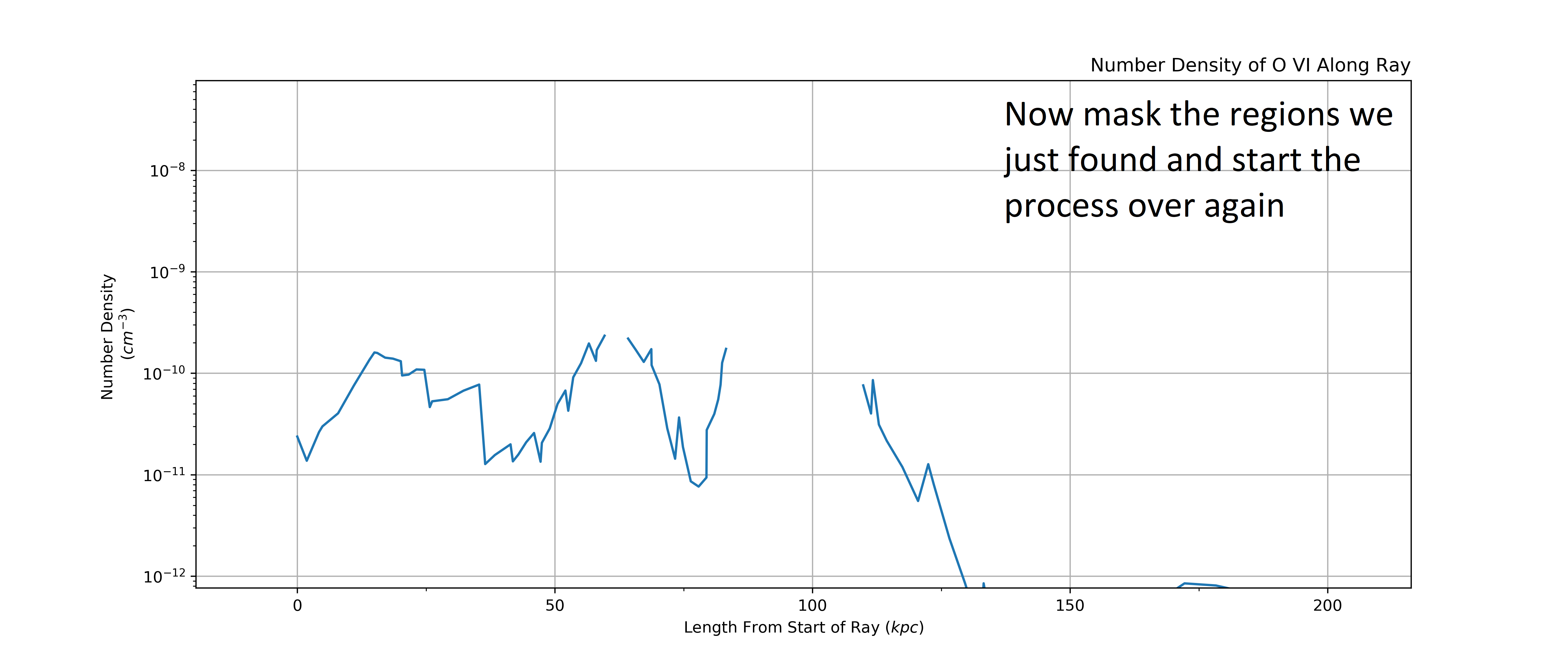
3.) Mask the intervals along the LightRay that were found in the previous step

4.) Repeat same step as (1.). Find the 80% cutoff based on the column density left over.

5.) define intervals just as (3.)

6.) Take all the intervals that have been found and sensibly combine all of them together. We do this by combining overlapping intervals if the average velocity of each intervals are within a threshold (set by velocity_res parameter. Default is 10 km/s)

7.) Now repeat process starting at step 3 until the total column density that is left over in the LightRay (ie not in an interval) is less than some the lowest detectable column density (set by min_absorber parameter. Default is Log(N)=13, though it can vary based on ion)

8.) Finally, we check whether each interval meets the detectable column density threshold. We return only the intervals that are above the threshold and define these to be our absorbers.

Detailed Example

If you want a better understanding of how the SPICE method works, here is a real life example. We break down each step of the method so you can see the under workings and see how some of the parameters may impact the algorithm.

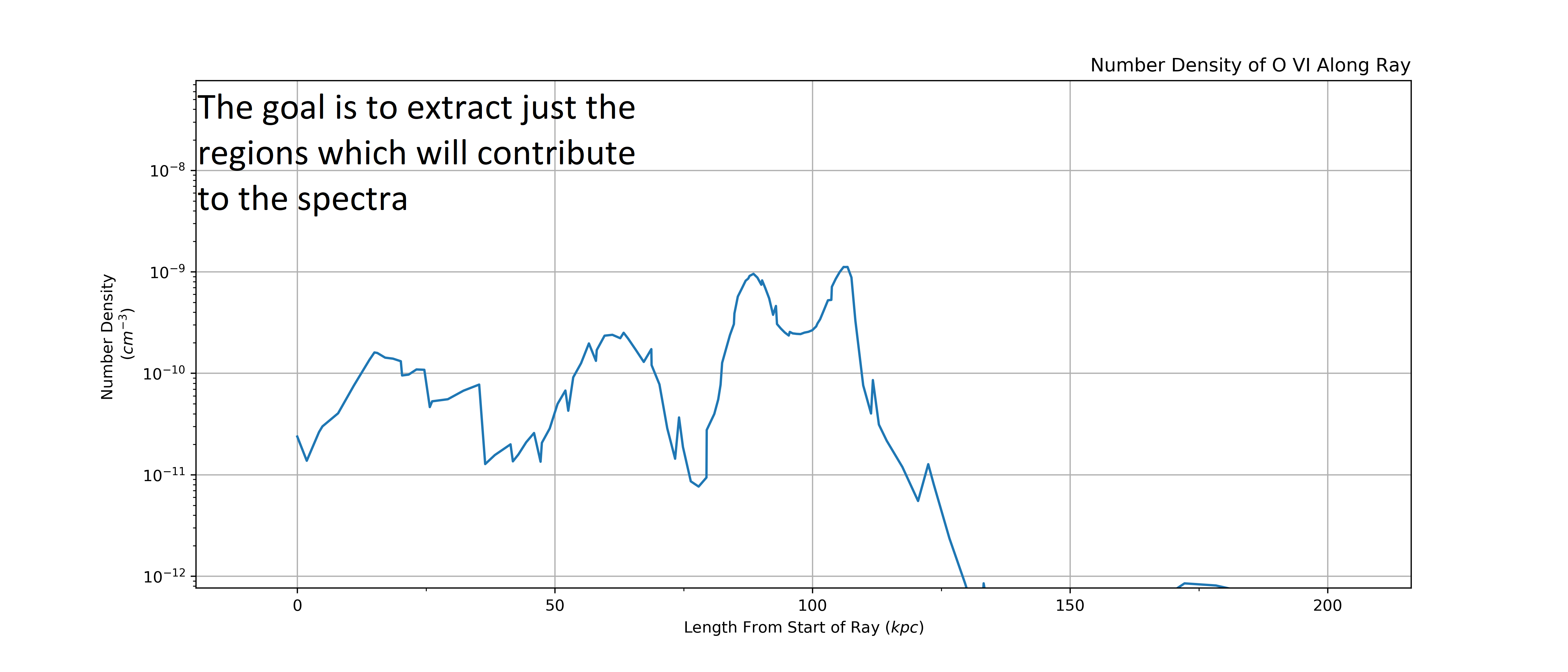
Here is our LightRay, looking at the number density of O VI along its length. Our goal is to find regions/intervals of cells along the LightRay with the highest column density and thus will meaningfully contribute to the absorption spectra of the LightRay.

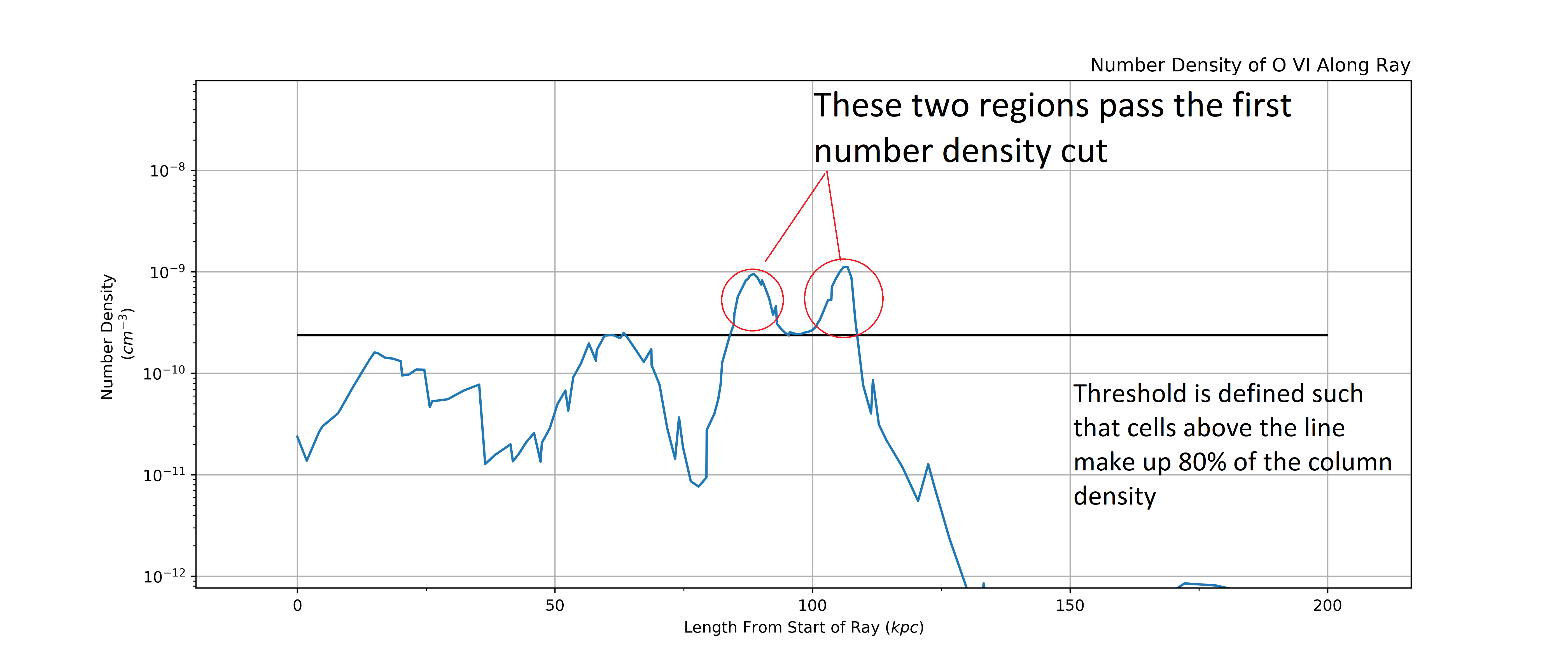
The first step is to find a cutoff value in number density such that cells above this cutoff make up 80% of the column density. This isolates the regions with very high number density. Below we can see two main regions that will likely be the largest absorbers.

Note

This 80% value is just the default value and can be tweak. We have found that the algorithm is fairly insensitive to this value. To change it, change the frac parameter in AbsorberExtractor

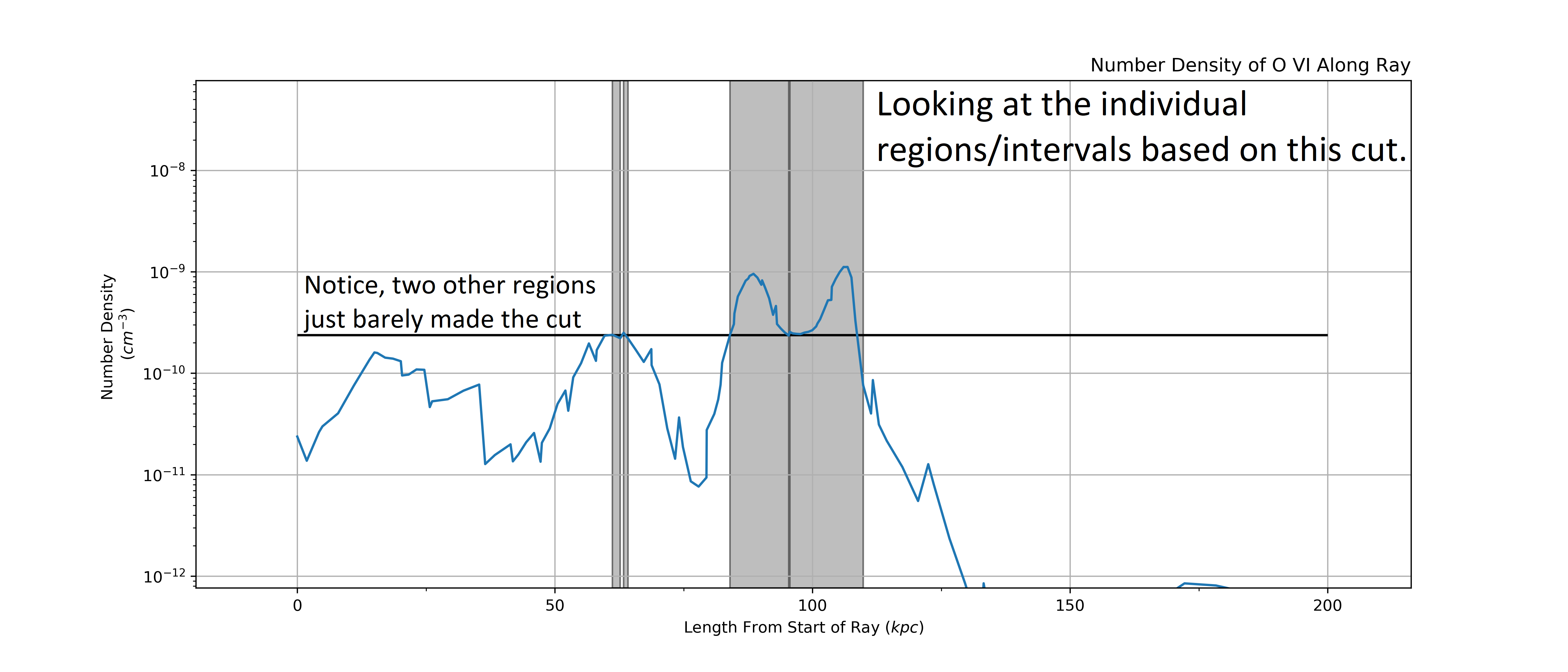
Next we define intervals that cover each region based on the cut. This leads us to 4 different regions, 2 small ones right next to eachother, and the two large ones that we could spot pretty easily from just eye balling it.

Now we mask the intervals we found witht he first cutoff and check there is enough column density remaining in the LightRay. We find there is LogN=13.3 remaining in the LightRay. We use a threshold for LogN=13 in this example so we continue to iterating through.

Note

The LogN=13 threshold is set by the absorber_min parameter. This sets the minimum detectable columne density for an absorber and so can vary based on ion and the research goals.

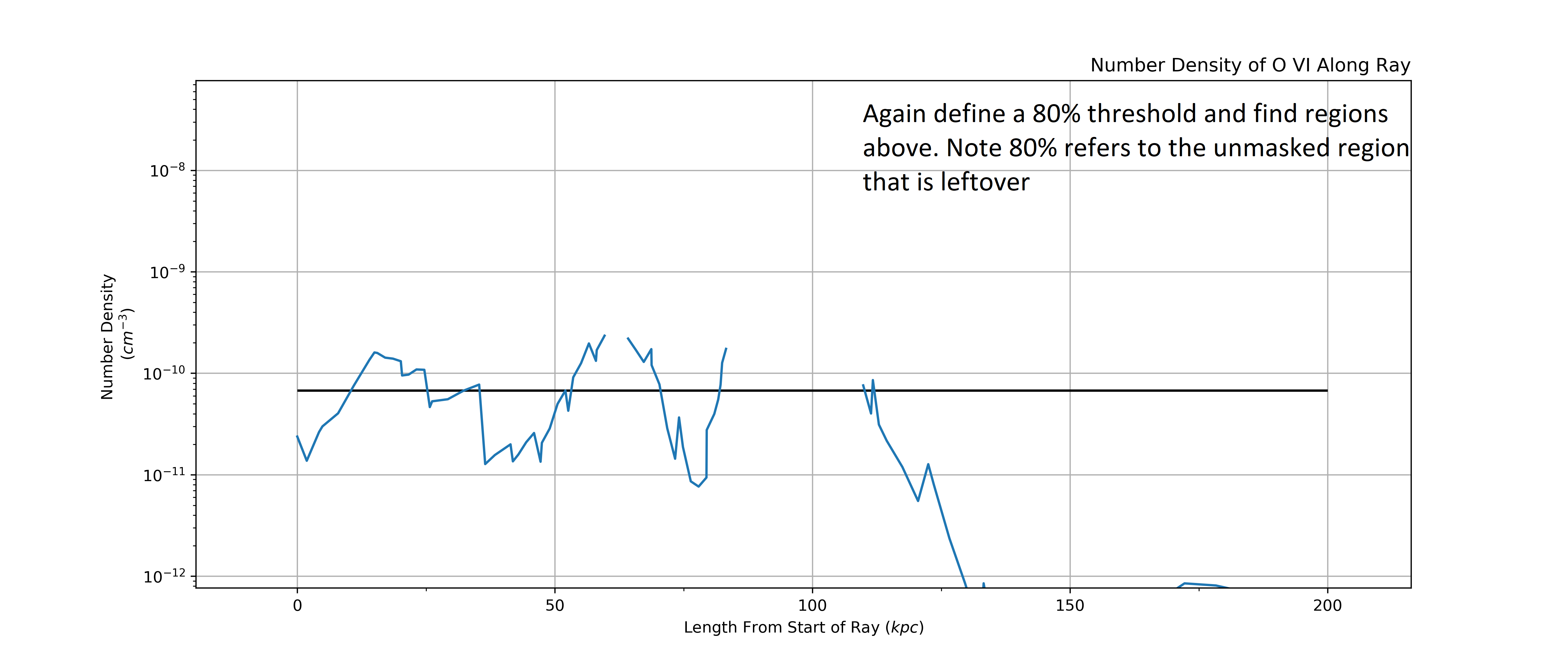
Here we define a new cut based on what is “left over” of the LightRay. This isolates some new regions that were at a lower column density but could still significantly contribute to the spectra, and so something we want to extract.

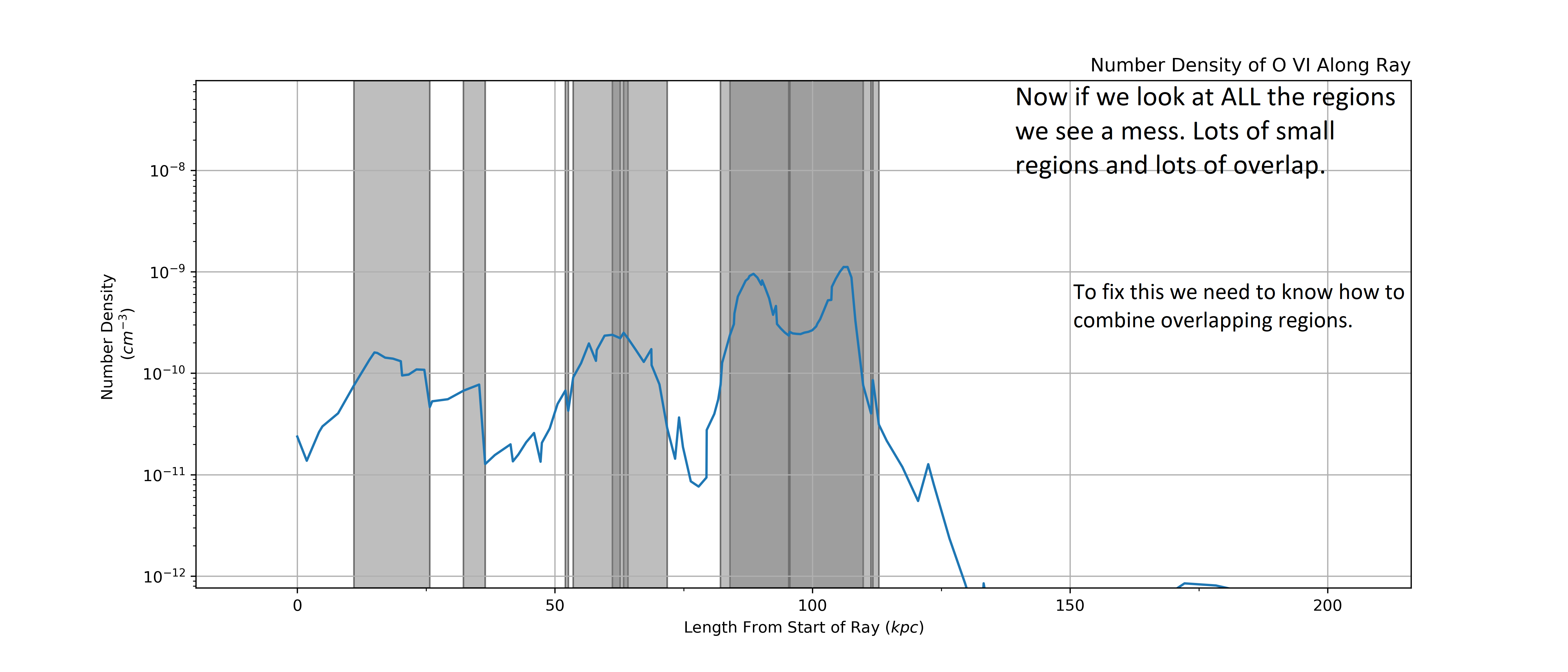
Again we extract intervals based on the cut. This time some of the intervals overlap masked regions. This is OK and will be dealt with in the “sensible combination” phase that comes next.

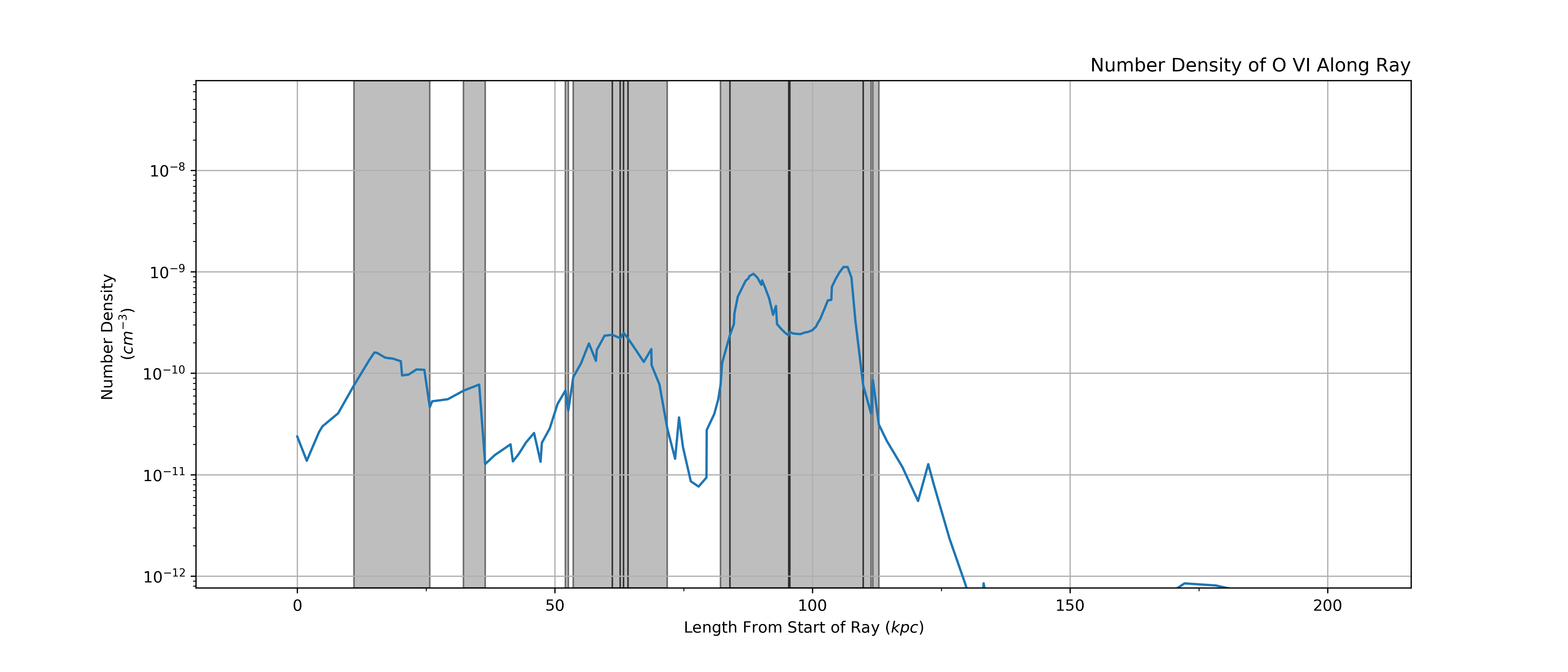
Combining all of the intervals from the two sets of cuts we are left with a bit of a mess. The first step is to divide up any regions with overlapping intervals into smaller component parts and then we will recombine them into sensible intervals that capture observationally distinct absorbers.

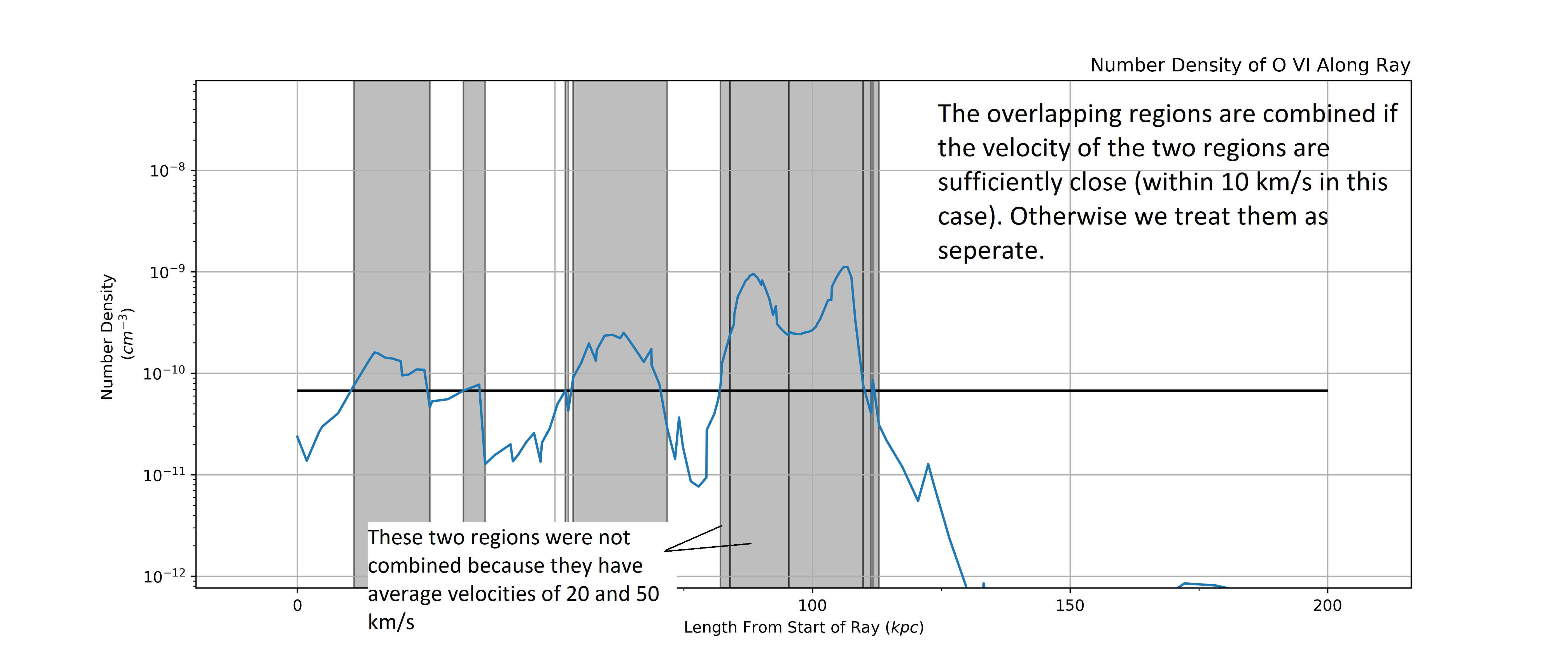
Now that we have separated the overlapping regions we can decide on which intervals to combine. We do this by taking into account the line of sight velocity information.

We calculate the average velocity of each interval and then combine two intervals if their velocities are with in a certain threshold, 10 km/s in this example.

Note

The velocity threshold that defines whether intervals/regions are combined is set by velocity_res. The value is motivated by the resolution of observed spectra though we have found the algorithm to be fairly insensitive to the precise value, especially when looking at a catalog of absorbers.

Here are the remaining intervals after our combining phase. You can see that some of the overlapping intervals were combined (like around 60 kpc) while others were separated/remained separated (like the two large absorbers at 100 kpc were not combined and some small ones on either side where not combined).

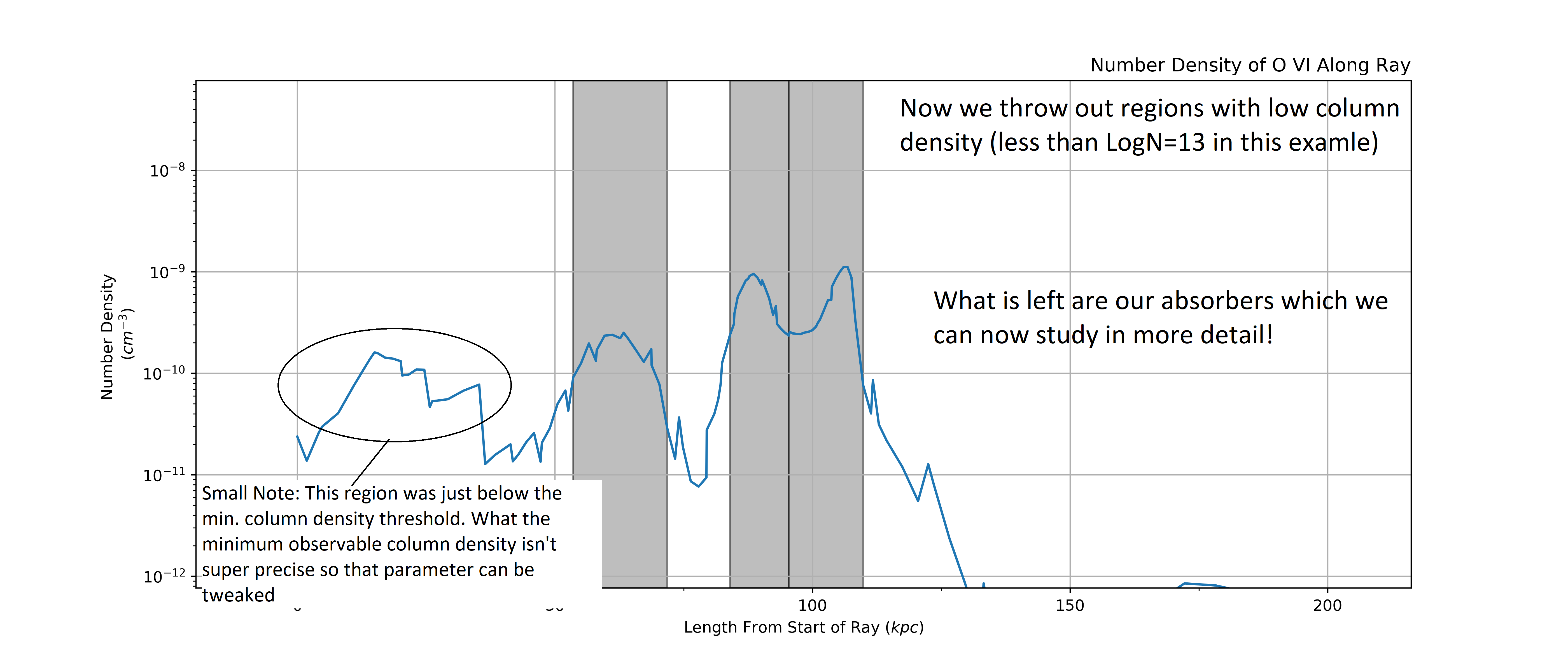
Now we again mask the regions with intervals and calculate how much column density is “left over”. In this case we find that there is only LogN=12.7 which is beneath our minimum absorber threshold of LogN=13.

So, we stop iterating through the ray and do a final cleanup of the intervals by throwing out all the intervals with “low column density” (based on absorber_min). This leaves us with the absorbers which can be further studied by extracting other information about them (e.g. temperature, radial velocity, metallicity, etc.).