Annotated Examples
One of the main goals of SALSA is to make it easy to construct a catalog of absorbers that can then be further analyzed. This process is broken into two steps, as demonstrated in the Identifying Absorbers example. SALSA also provides tools for combining these steps into one as shown in the Catalog Generation example.
Identifying Absorbers
Finding absorbers along lines of sight requires two steps: generating light rays and extracting absorbers. These two steps can be completed one after the other as shown in the following examples.
Step 1: Generate Light Rays
SALSA relies on the Trident package
to generate light rays that pass through a given simulation domain. These LightRays
are 1-Dimensional objects that connect a series of cells and save field information
contained in those cells such as density, temperature, and line of sight velocity.
From these we can then extract absorbers along these LightRays.
To aid in generating light rays, SALSA contains the
generate_lrays function which can generate any number of LightRays
which uniformly sample a given range of impact parameters. This can give us a sample that
is consistent with the samples of observational studies and prevents any
sampling bias when doing comparisons.
To get started we need to get a dataset. The one used in this example can be downloaded from yt.
To use this function first create a directory to save rays::
$ mkdir my_rays
Now we can load in a dataset and define some of the parameters that we will look for:
import yt
import salsa

# load in the simulation dataset
ds_file = "HiresIsolatedGalaxy/DD0044/DD0044"
ds = yt.load(ds_file)

# define the center of the galaxy
center = [0.53, 0.53, 0.53]

# the directory where LightRays will be saved
ray_dir = 'my_rays'
n_rays = 4

# Choose what absorption lines to add to the dataset as well as additional
# field data to save
ion_list = ['H I', 'C IV']
other_fields = ['density', 'temperature', 'metallicity']
units_dict = {'density': 'g/cm**3', 'temperature': 'K', 'metallicity': 'Zsun'}

# the maximum distance a LightRay will be created (minimum default to 0)
max_impact = ds.quan(15, 'kpc')
With the parameters set up we can now generate the LightRays. We will set the
NumPy seed used to create the random light rays so we can reproduce these results:
# set a seed so the function produces the same random rays
# SALSA uses numpy.random internally
import numpy as np
np.random.seed(18)

# Run the function and rays will be saved to my_rays directory
salsa.generate_lrays(ds, center, n_rays, max_impact,
                     ion_list=ion_list, fields=other_fields,
                     ray_directory=ray_dir)
Step 2: Extract Absorbers
SALSA currently supports only one method for extracting absorbers;
the SPICE method. To do this, we use the SPICEAbsorberExtractor
class. For more details on absorber extraction see Absorber Extraction Methods.
Now let’s extract some absorbers from one of the light rays we made:
ray_file = f"{ray_dir}/ray0.h5"

# construct absorber extractor & load our ray
abs_ext = salsa.SPICEAbsorberExtractor(ds, ion_name='H I')
abs_ext.load_ray(ray_file)

# use SPICE method to extract absorbers into an Astropy QTable
table = abs_ext.get_current_absorbers(fields=other_fields, units_dict=units_dict)
print(table)
name   wave   redshift      col_dens      ...        density            temperature        metallicity
     Angstrom               1 / cm2       ...        g / cm3                 K
---- -------- -------- ------------------ ... ---------------------- ----------------- --------------------
 H I  1215.67      0.0  6116814645533.102 ... 1.6863708884078385e-28 96469.46167662967 0.014059433622242793
 H I  1215.67      0.0 2505355090554556.5 ...   9.49051901355937e-28 50877.73530956685  0.01429726085432313
 H I  1215.67      0.0  9408651484697.451 ... 1.6823168463953486e-28 94252.62895133752 0.014273053208746916
Note
The metallicity column doesn’t have a unit listed even though we specified
via the units_dict argument that metallicity should be presented in "Zsun".
This is because of differences between the unyt package, which yt uses to
handle its datasets and the astropy package, which is used to construct the table.
These two package have different ways of treating “dimensionless” values such as "Zsun".
Fear not; the specified units can still be found via the table’s metadata:
table.meta["dimensionless_field_units"]["metallicity"]
To extract absorbers from multiple LightRays you can use the
get_all_absorbers function.
This will loop through a list of rays and
extract absorbers from each one:
ray_list = [f"{ray_dir}/ray0.h5",
            f"{ray_dir}/ray1.h5",
            f"{ray_dir}/ray2.h5",
            f"{ray_dir}/ray3.h5"]

# initialize a new AbsorberExtractor for looking at C IV
abs_ext_civ = salsa.SPICEAbsorberExtractor(ds, ion_name='C IV')
table = abs_ext_civ.get_all_absorbers(ray_list, fields=other_fields, units_dict=units_dict)
print(table)
name   wave   redshift      col_dens      ... interval_start interval_end LightRay_index
    Angstrom               1 / cm2        ...
---- -------- -------- ------------------ ... -------------- ------------ --------------
C IV 1548.187      0.0 113534735506095.75 ...            201          224              0
C IV 1548.187      0.0  39385046049917.84 ...            110          125              2
C IV 1548.187      0.0  42223273159161.47 ...            139          155              2
To retain information on where each absorber came from, a LightRay_index is
given. The number represents the ray it was extracted from. So all absorbers
extracted from ray2.h5 would have an index of 2. This can be useful for
comparing/analyzing absorbers on the same sightline.
Catalog Generation
To generate a full catalog of absorbers we can use the
generate_catalog function combine LightRay generation and
absorber extraction into a single step:
# Setup a fresh run
np.random.seed(18)
new_ray_dir = 'my_rays/catalog_rays'

catalog = salsa.generate_catalog(ds, n_rays, new_ray_dir, ion_list, method='spice',
                                 center=center, impact_param_lims=(0, max_impact),
                                 fields=other_fields, units_dict=units_dict)

print(catalog)
name   wave   redshift        col_dens             delta_v          vel_dispersion   ... interval_end        density            temperature         metallicity      lightray_index
     Angstrom                 1 / cm2               km / s              km / s       ...                     g / cm3                 K
---- -------- -------- --------------------- ------------------- ------------------- ... ------------ ---------------------- ------------------ -------------------- --------------
 H I  1215.67      0.0     6116814645533.102  14.186900060851054 0.38448653831790686 ...          204 1.6863708884078385e-28  96469.46167662967 0.014059433622242793              0
 H I  1215.67      0.0    2505355090554556.5  -1.030940550779623  5.6651802667616105 ...          222   9.49051901355937e-28  50877.73530956685  0.01429726085432313              0
 H I  1215.67      0.0     9408651484697.451 -26.728157177393342    5.20649247388288 ...          226 1.6823168463953486e-28  94252.62895133752 0.014273053208746916              0
 H I  1215.67      0.0 4.768813058817296e+18  108.06531773144404  1.5094660329566112 ...          156 1.4855073194776734e-26 16302.538383554222  0.01419281650535469              2
C IV 1548.187      0.0    113534735506095.75 -2.2526205975043787  13.699041596403035 ...          224  8.916084054641148e-28  53985.90647005775 0.014287622611506724              0
C IV 1548.187      0.0     39385046049917.84  116.44013343087262   6.581810678140516 ...          125 3.9893530708657154e-27  29972.84586437622 0.014338369933268647              2
C IV 1548.187      0.0     42223273159161.47  115.32578395061917   3.072995936488675 ...          155  3.326550307789238e-27  34632.02222613203 0.014263515932284202              2
Note that we make a new directory for this example. That’s because
generate_catalog looks first to see if rays have been created in the given directory.
If there are the right number of rays and they all contain the right ions and
other fields that were specified (in this case that would be 'density',
'temperature', 'metallicity'), then those rays will be used. Otherwise, new rays are
created using generate_lrays.
Next, get_absorbers is used to find the absorbers from each ion
in ion_list and finally a catalog is returned as a pandas.DataFrame. Note
that the lighray index is unique only up to the ion/wavelength
Visualizing Absorbers
To visualize what is actually being extracted from the LightRay objects,
you can use the AbsorberPlotter class. This class accepts an
AbsorberExtractor object to have access to the extracted absorbers.
To get a full picture of what is happening at each level we can create a multi panel plot containing:
A slice of the simulation with the ray annotated
The number density profile along the ray’s path
The line of sight velocity profile along the ray’s path
The synthetic spectra created from the ray
This figure gives you a good overview of what is happening and can give valuable
context to the absorption extraction methods. Additionally, each panel can be made
individually if you care less about the spectra or don’t want to plot a slice;
see the AbsorberPlotter API for options.
To create the multi-panel plot:
import salsa
import yt
import matplotlib.pyplot as plt

# Assuming we've already generated some rays, extract absorbers
ds = yt.load("HiresIsolatedGalaxy/DD0044/DD0044")
abs_ext = salsa.SPICEAbsorberExtractor(ds, ion_name='H I')
abs_ext.load_ray("my_rays/ray0.h5")
abs_ext.get_current_absorbers()

# set the y limits for one of the plots
num_dense_min = 1e-11
num_dense_max = 1e-5

# Plot!
plotter = salsa.AbsorberPlotter(abs_ext)

fig, axes = plotter.plot_multiplot(outfname='example_multiplot.png',
                                  center = [0.53, 0.53, 0.53],
                                  num_dense_max=num_dense_max,
                                  num_dense_min=num_dense_min,
                                  make_spectra=False)
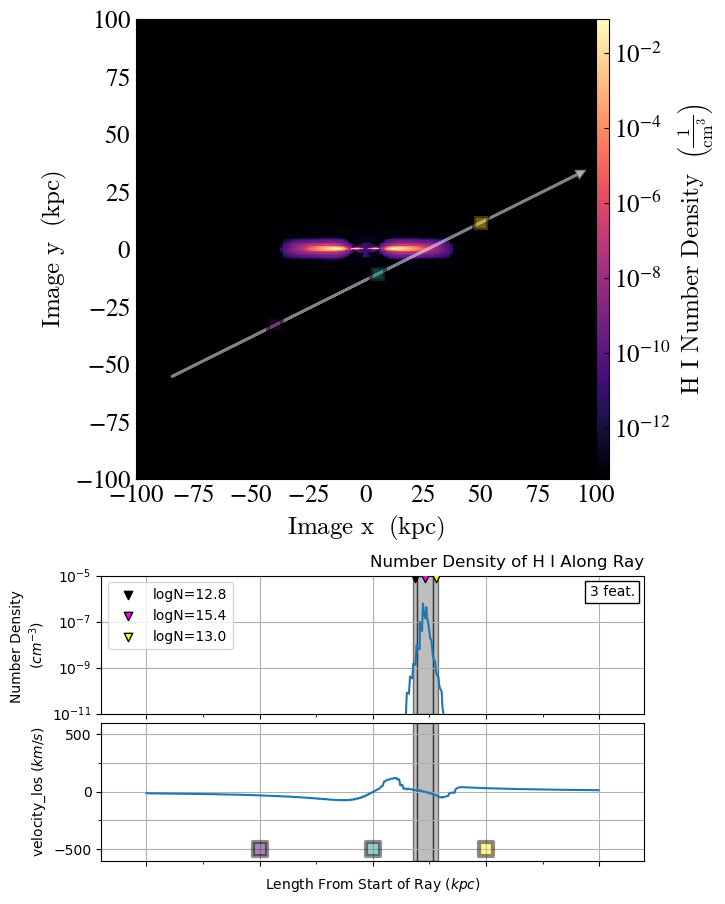
The grey regions on the middle two plots indicate the absorbers that the SPICE method finds. The three highest column densities are marked and displayed in a legend.
Warning
While SALSA can include the Trident spectrum in these multiplots, there is currently an issue with Trident’s spectrum generation due to changes in the underlying yt module. See the associated (GitHub issue)[https://github.com/trident-project/trident/issues/217].